


 TRAINING


 PAPERS
 REFERENCES
 GET IN TOUCH

|

|
 Downloads
|
 Prices
|
 Videos
|


|
"I love Petrophysics" |
GeolOil - A modified Pickett plot equation for shaly sands
By: Oscar Gonzalez, GeolOil LLC. This paper was first published on June 2021 on the website geoloil.com
This article presents an equation to simultaneously estimate the rock's porosity cementation exponent m, and the formation water resistivity Rw. The classic Pickett plot equation allows to estimate m and Rw, but only works on clayless rocks, like clean sands and carbonates. The modified Pickett plot equation allows to estimate m and Rw both on clean sands and on shaly sands with conductive matrices. The extended equation reduces to the regular Pickett plot equation when Vshale=0.
The math of the original regular Pickett plot equation
The classic, regular Pickett plot equation for clean rocks is deduced from the SW Archie equation:

where:
- SW is the rock's water saturation
- Rt is the true or un-invaded deep resistivity
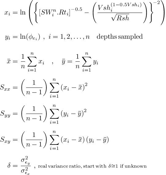
- φ is the rock's porosity. Since we are dealing so far with clean rocks, the total porosity and the effective porosity are the same: φ = φt = φe, likewise, SW = SWt = SWe either in the total or in the effective pore space.
- Rw is the formation water resistivity, or the water resistivity in the effective pore space
- a≃1 is some times called a "tortuosity" empirical multiplier factor always accompanying Rw, occasionally needed to improve accuracy and achieve a better fit.
- m≃2 is the porosity exponent, usually called the cementation exponent, and
- n≃2 is the saturation exponent.
After taking natural logarithms ln() (base e=2.71828...) and re-arranging terms, the Archie SW equation can be written as a linear equation on the terms ln(Rt) and ln(φ): (common logarithms log10() could also be taken instead)

The Pickett plot equation for clean rocks after re-arranges becomes:

 For graphical purposes, a plot on a base 10 log-log scale is traditionally used:

Modifying the Pickett plot equation for shaly sands
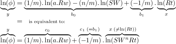
The Pickett plot equation on coefficients b0 and b1, can also be re-written as another linearized expression with coefficients c0 and c1:
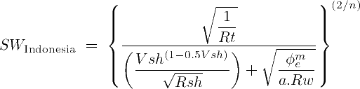
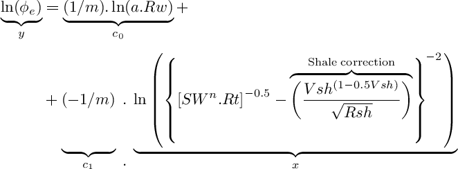
To deal with shale content, we can no longer use the Archie equation for clean rocks. A water saturation for shaly sands must be used instead. Let's choose the Indonesia Poupon-Leveaux water Saturation Equation (which is an overall good model for shaly rocks):
After some algebraic operations, the Indonesia SW equation can be linearized on coefficients c0 and c1. Then, a modified Pickett plot equation for shaly rocks is obtained. Notice that the equation is reduced exactly to the regular Pickett plot equation when Vsh=0. That is, the shale correction would become 0.
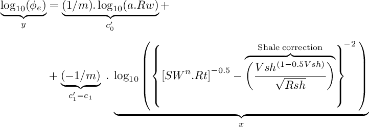
For graphical purposes, a plot on a base 10 log-log scale may be used:
Solving the parameters m and Rw
In the former equation, y = c0 + c1.x, the "independent" variable x
is no longer a stable, well known, reliable measurement of ln(Rt). It is instead better to consider x
as a random variable that depends on somewhat inaccurate measurements of Rt, and
erratic and noisy estimates of SW, and Vsh.
That's it, x = f (Rt, Vsh, Rt) is itself a Random variable, and conventional
Simple Linear Regression
is not an appropriate model. Notice also that a graphical 2D classical solution plot on two variables
x=ln(Rt), and y=ln(φ), no longer applies. A graphical representation would need a 4D
dimensional space, or a least a 3D space if SW=1 can be assumed constant if applied in a water body.
A model based on errors on both variables x and y, was popularized by Edwards Deming in 1943, and is called Deming regression (a case of orthogonal regression). Its probabilistic solution is:
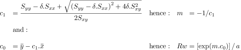
where:
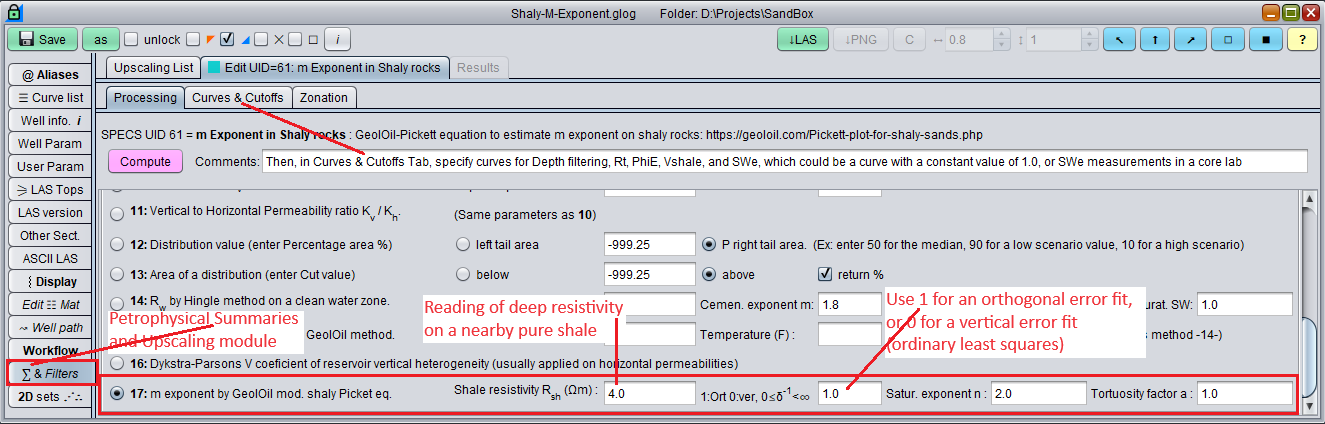
The GeolOil panel to estimate the m porosity cementation exponent on shaly rocks
Applying the general solution
The developed equations have a general applicability, and reduces to the standard Pickett-Plot equation for clean rocks when VSH=0. In some reservoirs, a high scatter dispersion on the data, uncertainty, and not accurate or poorly calibrated log curve signals, easily leads to cloud pattern cross-plots instead of clearly sharp linear trends with low r2 determination terms. In such cases, it would be better to assume or estimate first a formation water salinity or Rw first, and then estimate m through other method.
Also follow these guidelines when applying the technique:
-
Clean rocks in water bodies(the original Pickett plot approach)
Seek for clean rocks in water bodies like aquifers and water pockets, then set Vshi=0, and SWi=1. This may yield small sample sizes n, specially when dealing with sandstones instead of carbonates. A traditional simple linear regression may produce too large values for the m exponent. The Deming regression shown above controls the error orthogonality and might deliver a more reasonable estimate for m when the parameter δ-1 is set close to 1.0 Use δ-1=0 for a conventional ordinary least squares simple regression that minimizes vertical residual errors in y=log(φe) -
Shaly sandstones in water bodies
In water bodies like aquifers and water pockets, seek for clean sandstones and moderate shaly sandstones (say Vshi ≤ 0.30). Skip shales and very shaly sandstones (say Vshi > 0.30) that would yield φe≃0 and huge negative values for ln(φei). Then set SWi=1.
Notice that the acceptance of shaly sandstones increases the depth's collection sample size n, producing a more representative porosity heterogeneity, and a more stable, better estimate for m. The technique works as long as Vsh is carefully estimated from gamma ray or neutron-density porosity difference. -
Reservoirs with core lab data(even in pay zones)
If there are quality core lab measurements of SW<1, we are no longer restricted to apply the equation on water bodies with SW=1. Of course, make sure that core SW<1 values are reliable, and core depths are properly shifted to match log depths. Then merge the collection of core samples with potential log depth zones in water bodies.
Regarding core porosity measurements, carefully assess its representativeness in shaly rocks. Core porosity may be measured using helium, which could enter into the clay internal pore space, and hence measures more the total porosity φt instead of the required effective porosity φe.
We suggest to keep core lab measurements only of the water saturation SWi<1, tie them with log properties of Rti and Vshi at their depths, and merge this collection with log depths in water bodies SW=1 if available. The use of core data SWi relieves the need to search for water bodies. Not always we have reservoirs with aquifers and water pockets to assume SW=1.

|
Related articles:
|
|
| |


|
|
|
© 2012-2026 GeolOil LLC. Please link or refer us under Creative Commons License CC-by-ND |