Downloads

Prices

Videos

Products

Consulting

Training

About

Contact

4.7 ★ on Google

Consulting

Contact

More ☰

GeolOil - Logging Scripting (GLS) Reference Manual and API Documentation

"If you can code in GLS and Groovy, then there will be no limit to GeolOil's capabilities."
Enis Aliko. Senior Drilling Engineer. Wellynx. Italy.∎

The GeolOil GLS is a simple and concise scripting programming language specifically designed to process petrophysics LAS files. It allows easy handling of well log curves without worrying too much about invalid blank, or missed -999.25 values. Some minimum exposure to elementary scripting is advised. Please read the GLS log scripting tutorial introduction before checking this reference material.

The Java methods print() and println() are compatible with GLS, which are essential to debug scripts. For instance, this snippet of code prints integers from 1 to 10:
for (int i=1; i<=10; ++i) {println (i);}

@ Curve references and % Parameter References

If Measure Depth is the well log Curve number 1, then the syntax: MD = @1 defines the Curve object that represents that curve. Like wise: PhiE = @17 defines the object that represents effective porosity at the curve number 17. Notice that the Sigil @ is prepended to the curve number.

User aliases can be used as references to curves. For instance, if the volume of shale is the curve number 23, VSH = @23 still defines the curve. But if the volume of shale curve has been aliased as @Vshale, then the code VSH = @Vshale refers to the volume of shale (regardless of its curve number), which is the preferred notation. Original curve references are usually placed at the beginning of the script, but they can be placed everywhere before they are used.

Similarly, named constants are prepended with the Sigil %. For instance, if the log User Parameters section contains in its table the entry: Salinity 43000, the code NaCl = %Salinity grabs the value 43000 from the section. The sigil % reads in order of priority the log sections: Tops, User Parameters, Well Parameters, and Well Info. The first match found is the one kept, avoiding thus any possible repetition.

GLS Instance Functions

The following functions are applied on Curve objects, and curve represents an instance of the object:

curve.get(depthIndex) Returns the value or signal of the curve at a depth index
curve.set(depthIndex,value) Sets a value at the depth index
curve.getIndexFromDepth(depth) Gets the depth index that corresponds to a given depth
curve.getSignalFromDepth(depth) Gets the curve signal or value that corresponds to a given depth
curve.blank() Returns a blank curve with void -999.25 values in each depth index
curve.size() Returns the size, or the number of depth index cells of the curve

curve.quantile(leftArea) Returns the quantile for the whole curve. To get a classic P50% scenario, use curve.quantile(0.5). To focus on the distribution low (left) value that corresponds to the 10% left area, use curve.quantile(0.10). The user must ensure that not interesting depths or zones, should be excluded by setting void -999.25 blanks at those depth indexes.

curve.interpolate() Fills the blank -999.25 void gap values of curve with an interpolation. A GeolOil proprietary interpolation algorithm default curvature=0.5 parameter is internally used: read the next method for details.

curve.interpolate(curvature) Fills the blank -999.25 void gap values of curve with an interpolation. The curvature parameter [0.0 to 1.0] specifies how straight or smooth the resulting interpolated curve will be. A value of 0.0 yields a linear interpolation, the default 0.5 recommended value yields reasonably smooth results that never produce outliers. The value of 1.0 yields the most smoothed curve with continuum 1st and 2nd derivatives, but easily produces out range outliers, useless for most petrophysical properties.

curve.interpolate(gap,curvature) Fills the blank -999.25 void gap values of curve with an interpolation. The gap parameter specifies the maximum depth gap to fill with an interpolation. For instance, a gap of 10.0 will interpolate results for internal depth separation distances of 10 ft (or meters) or less, but will not fill (leave untouched) void -999.25 points separated at depth distances of more than 10 ft. The curvature parameter behaves as explained in the former method.

GLS Stream Operators

The operators +, -, *, /, are normal binary operators that can take either a scalar or a log curve to the left or right side of the operator. The power operator is ^. For instance, x^y means x^y. Operators are evaluated from left to right according to standard operator precedence priority as any programming language. To change the evaluation order, just use enough parentheses.

The character or sigil @ is reserved for curve number and alias references. The character or sigil % is reserved for named constants. For example, if deep resistivity is the curve number 13, the assignation Rt = @13 defines the variable Rt as a whole curve object. Measured depth should normally be the first curve on a LAS file, so MD = @1 defines MD as the curve 1. To separate instructions use ;. To start a remark or a comment to be omited use #.

The internal representation for missed, dummy, unknown, blank, invalid, infinite, not a number, or any irregular number is -999.25. GeolOil GLS handles all cases automatically in the stream mode (it compiles and executes for you all necessary depth loops on curves and if conditions), but some manual control is needed on the regular looping mode when using comparisons like ==, <, ≤, >, and ≥.

GLS Stream Functions

A stream function is automatically applied to a whole log curve. It internally takes care of all depth cells, looping, and properly handling of invalid dummy and -999.25 values. A special algebra handles automatically a whole curve without any need to loop inside individual depth values. All functions can be applied to either scalars (a single value), or log curve arguments:

abs(x) Returns the absolute value or argument x

Exponential and logarithmic functions:

exp(x) Returns e^x
ln(x) Returns the natural logarithm (base e=2.71828...) of x
log10(x) Returns the common logarithm (base 10) of x

Trigonometric functions:

sin(x) Returns the sine of x, where x is in radians, not degrees.
cos(x) Returns the cosine of x, where x is in radians.
tan(x) Returns the tangent of x, where x is in radians.
asin(x) Returns the inverse function sin^-1(x). The returned result is in radians, not degrees.
acos(x) Returns the inverse function cos^-1(x). The returned result is in radians.
atan(x) Returns the inverse function tan^-1(x). The returned result is in radians.

Pre-multiplier Functions.

log scripting

ind(x,y) Returns 1 if x < y. Returns 0 if x ≥ y. Returns -999.25 if either x or y are invalids or -999.25
ind(x,y,z) Returns 1 if (x ≤ y) and (y < z). Returns 0 if condition is false. Returns -999.25 for invalid arguments

blank(x,y) Returns -999.25 if x < y. Returns 1 if x ≥ y. Also returns 1 if either x or y are invalids or -999.25
blank(x,y,z) Returns -999.25 if (x ≤ y) and (y < z). Returns 1 if condition is false. Also returns 1 for invalid args
blankOutside(x,y,z) Returns -999.25 if y lies outside the interval: x ≤ y < z. Returns 1 if y lies in the interval, and also 1 for invalid arguments

Optimization and error functions:

MSE(x,y) Returns the Mean Square Error difference between the curves x & y
MSE(x,y,w) Returns the Mean Square Error difference between the curves x & y. The difference is weighted through the curve w.

RMSE(x,y) Returns the Root Square of the Mean Square Error difference between the curves x & y. It has the intuitive advantage over MSE, that the result bears the same unit as the original curves. The result is equivalent to the expression (MSE(x,y))^(0.5).
RMSE(x,y,w) Returns the Root Square of the Mean Square Error difference between the curves x & y. The difference is weighted through the curve w.

Special functions:

getIndexFromDepth(x,depth) Returns the depth index that corresponds to a depth for the curve x. This function is also available as an instance function
getSignalFromDepth(x,depth) Returns the curve signal or value that corresponds to a given depth for the curve x. This function is also available as an instance function

isValid(x) Returns 1 if x is a valid argument, 0 if x is invalid, blank, or missed like -999.25, NaN, infinite, etc.
valueOrZero(x) Returns its original argument x, if x is valid. But returns 0 if x is invalid

trim(left,x,right) Returns x, if left ≤ x < right. Returns left, if x < left. Returns right if x > right. Returns -999.25 for invalid arguments

stretch(x,HashMap<Double,Double>()) Vertically stretches or compresses the curve x to match a mapped depth of marker correlations OriginalTopDepth → TargetTopDepth. (see advanced scripting). It produces a new curve.

calibrate(x,HashMap<Double,Double>()) Calibrates the signal of the curve x (the curve values are stretched or contracted) to match the trend of a mapped depth of curve Signal → CalibratedSignalValue. It produces a new curve.

shiftCurve(x,n) Vertically shifts the curve x downwards n depth steps if n > 0, (producing a deeper curve), or upwards n depth steps if n < 0: It returns a new shifted curve
shiftLeft (x,cutoff,replacement) Horizontally shifts the curve x: where (x < cutoff) set (x = replacement). It returns a new different curve
shiftRight(x,cutoff,replacement) Horizontally shifts the curve x: where (x > cutoff) set (x = replacement). It returns a new different curve

min(x,y) Returns the smaller of x and y, or -999.25 if either x or y are unknown, missed, invalid or -999.25.
min(x1,x2,x3,...,xn) Returns the smallest of x₁, x₂, x₃, ..., x_n. Returns -999.25 if an argument is invalid, missed, or -999.25.

max(x,y) Returns the larger of x and y, or -999.25 if either x or y are unknown, missed, invalid or -999.25.
max(x1,x2,x3,...,xn) Returns the largest of x₁, x₂, x₃, ..., x_n. Returns -999.25 if an argument is invalid, missed, or -999.25.

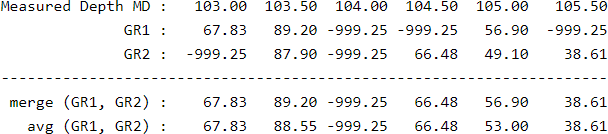
merge(x,y) Returns x, if x is known. Returns y, if x is missed, invalid, unknown or -999.25 (transparency): merge puts the x curve on top of y
merge(x1,x2,x3,...,xn) Returns a new merged curve from x₁, x₂, x₃, ..., x_n. Top priority curve is x₁. If x₁ is missed, x₂ is taken and so on

avg(x,y) Returns the arithmetic average of x and y. Any -999.25 missed value is skipped. Only returns -999.25 if both x and y are missed.
avg(x1,x2,x3,...,xn) Returns the average of x₁, x₂, x₃, ..., x_n. Any missed value is skipped. Only returns -999.25 if all values are missed.

merge()

avg()

GeolOil concept to merge LAS well log curves

User Defined Stream Functions

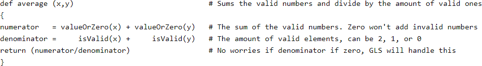
In some cases the built-in collection of GLS functions is not enough for some advanced computations. Custom specific functions can be defined by the user both in stream mode or regular depth looping mode. The defined functions are usually placed at the end of the script. As an example, the following user defined stream function has the same behaviour as the default built-in GLS avg(x,y) function:

GeolOil GLS Script example to define a function

GLS Regular Depth Looping Mode

The GLS stream mode normally handles most of the programmer's needs. However, in some cases an advanced user may want full control of the computations depth by depth step on a curve. Such custom scripts are usually unnecessarily verbose, long, complex, and prone to bugs, as the user has to take care of all cases, exceptions, if conditions, and looping.

While algebra with invalid numbers like NaN or -999.25 is handled correctly by GLS, the user must not use if and comparison operators like <, ≤, ==, ≥, or >. The reason for that is that an unknown number like NaN or -999.25 can't be compared against anything by definition. For instance, what is the logic result of the instructions: x=-999.25; if (x<0) {x=x+1;}. Since -999.25 is a missed invalid number, don't expect the result to be true (yielding x=-998.25). Likewise, the if() comparison should not be taken as false either!. How to treat this then?

There are two work-arounds to deal with this problem. The first choice is prefer to script as much as possible in the GLS stream mode that takes those details correctly and automatically for you. The second choice is to explictly skip all invalid comparisons and continue to the next instruction or iteration in a depth loop using the isValid(x) function, or its logic negation !isValid(x)

Looping over all Depths

To build a loop over all depths in a LAS file, the user needs to take care of the followng details:

Define new void curves initialized to blank missed values (-999.25) that can store computation results. Once any curve is already defined, a new curve with -999.25 cell depths is easily assigned using the .blank() instance method on the LasCurve. For instance:
MD = @1; workingResult = new LasCurve (MD.blank());

Find the LasCurve size. Which is the amount of elements or depths in the curve, for example: nDepths = MD.size();

Get for each LasCurve to be read, its scalar individual value at the target depth index. This is done with the LasCurve instance method .get(i). For instance:

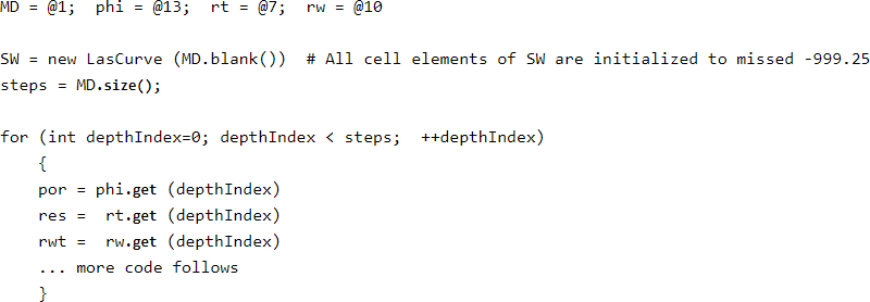
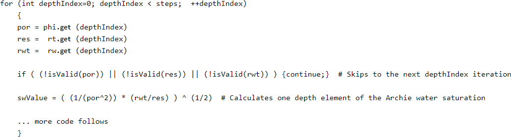
GeolOil GLS Script example to set a depth loop

Continue to the next loop iteration if you plan to use comparators <, ≤, ==, ≥, or >, on variables that might have missed -999.25 values which would behave unexpectedly during comparisons. Just use logical or on negated !isValid() functions to skip those possibilities. (If any value is invalid, skip and continue to the next iteration) For instance:

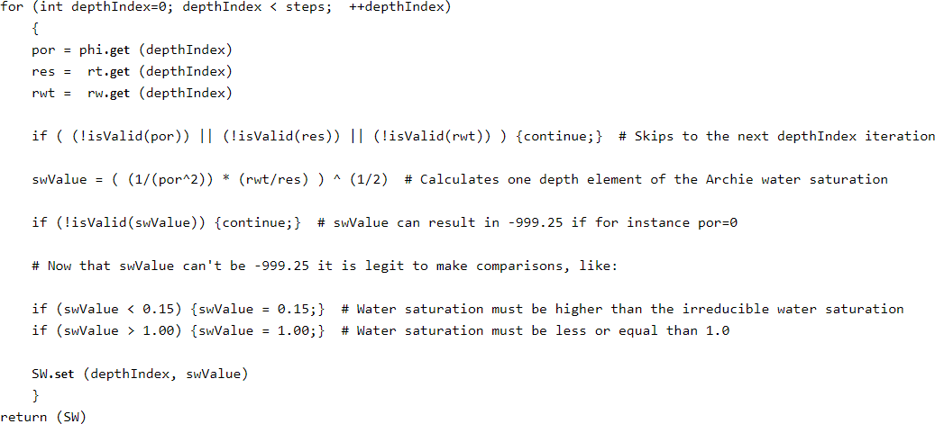
GeolOil GLS Script to compute water saturation SW in depth loop mode

Set the collected values of swValue in their corresponding whole SW LasCurve positions using the instance method .set (index, value):

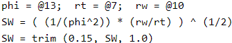
GeolOil GLS Script example to define a function

All this large boilerplate code is equivalent (and safer, more intuitive and human readable) to just only three lines of scripting in the Stream Mode. So think twice before considering to write code on the Regular Looping Mode, or other petrophysical software under Python scripts. What about trying in Excel?

GeolOil GLS equivalent short script in stream mode

Notice that the former script last line does not end with the command return(SW). An explicit return() command is optional. If the script does not find a return() command, the value of the last expression evaluated is returned, in this case SW. This makes the script more concise.

Only if you really need to write complicated math code that involves the flow control statements: if, else, for, do, while, continue, and break, stick with the Stream Mode.