GeolOil - How to estimate SWirr irreducible water saturation from well log curves

This article discusses practical techniques to estimate the SWirr irreducible water saturation of a rock, from commonly available or estimated well log curves like porosity, permeability, and shaliness. Laboratory measurements of porosity, permeability, and capillary pressure tests are needed to feed correlation parameters. The equations shown, rest on sources of available lab data for the particular reservoir under study. If there are no lab tests, a similar behavior for capillary pressure tests may be taken for an analogous reservoir, or assumptions need to be made.

The irreducible water saturation of a rock sample, is the minimum water saturation that is left in the rock after executing a laboratory process to extract the maximum possible amount of water through a displacement test. The connate water saturation of a reservoir rock is a similar concept, but at the natural reservoir conditions of its pressure and temperature, which is equivalent to the water saturation when the oil or gas saturation is maximum at the shallowest reservoir depth.

At the reservoir, it is usually assumed than in ancient geological times, the reservoir rock was fully impregnated with water. Then other fluids —typically oil and gas— migrated upwards by gravity, displacing water. Since at the controlled laboratory conditions, injection pressure and temperature might be set at higher values of those of the reservoir:   SWirr_(lab) ≤ SWconnate_(reservoir)

Mercury Injection Capillary Pressure Tests

A common lab technique to get a value of the irreducible water saturation of a rock sample, is the capillary pressure test through mercury injection (there are also centrifugue tests, and relative permeability tests). After preparing and cleaning the chosen rock sample with solvents like toluene, the sample is impregnated with brine water — ideally from the same formation water, or a similar prepared one with a close ionic salinity composition—.

Then mercury (Hg, a non wetting phase on its liquid state) is injected into the sample at increasing pressures, and the amount of expelled water is measured (and converted to saturation). The higher the pressure, the more expelled water (and less residual water saturation left in the rock). At some point, increasing the pressure has a small influence to further reduce the remaining water saturation. As seen on the legacy chart below: y=CapPress versus x=SW shows vertical asymptotes. The water saturation at the asymptote can not be reduced any more, and hence is considered the achieved irreducible water saturation.

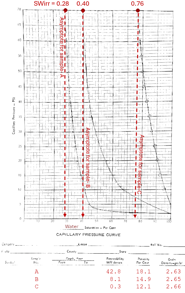
Legacy (year 1969) lab test results of capillary pressure curves measured on three rock samples

The definition of irreducible water saturation has its caveats. In some samples an obvious completely vertical asymptote is never reached (like the sample C above). Hence, the SWirr values are often overestimated. And also, for really big injection pressures, SWirr can be reduced more and more. Furthermore, the SWirr value also is smaller for longer durations of the tests, as the heavy mercury will have more time to patiently impregnate smaller pores.

Classic correlations between porosity and irreducible water saturation

The three most referred relationships between porosity and irreducible water saturation are:

1. The Buckles (1965) correlation between irreducible water saturation and porosity.


2. The Timur (1968) correlation between irreducible water saturation with porosity and permeability, and


3. The Holmes-Buckles (2009) correlation. A porosity powered extension of the Buckles correlation by the Holmes brothers: Michael, Antony, and Dominic, presented at the 2009 AAPG Convention in Denver. The Timur (1968) correlation reduces exactly to the Holmes (2009) correlation when the permeability can be approximated as a power-law function of porosity —the default correlation between permeability as a function or porosity—

The Buckles correlation for irreducible water saturation

The Buckles correlation is based on the hyperbolic Buckles plot, that states that the normalized bulk volume of irreducible water (BVWirr) is approximately a constant in a same rock type family:

BVWirr = φ . SWirr ≅ C = Constant

If there is a at least one capillary pressure lab test with a measured pair of   (φ_lab,  SWirr_lab)  values, the C constant is simply found by one multiplication —However, if there are several lab pair values, we better recommend to use the Holmes-Buckles correlation—. It is not difficult for an experienced geo-scientist to get some intuitive familiarity between a porosity and its corresponding irreducible saturation value. In absence of lab data, GeolOil software defaults as (φ_lab,  SWirr_lab)  ≅  (0.10, 0.25). For quick and dirty sensitivity explorations, the user could keep fixed a porosity of say 10%, and play with possible SWirr educated guess candidate values.

It has to be noted that the Buckles correlation is only approximately valid around the neighborhood of the range of measured lab tests. For example, if   (φ_lab,  SWirr_lab)  ≅  (0.10, 0.25)  , C = 0.025 = BVWirr  , and therefore  SWirr ≅ 0.025 / φ. This expression is completely unusable for low porosities. For instance, a tight rock porosity of 1% (φ=0.01) will yield  SWirr=2.5 >>1.0 , a completely unacceptable result, whose correct value should be close to SWirr≅1.0 (100%), as it would be quite difficult to displace residual water on such tight rocks.

That is, the Buckles correlation suffers severe, inadmissible overflow boundary extrapolation effects. The Holmes-Buckles correlation suffers either overflow or underflow, depending upon its power slope parameter. While overflow could be alleviated by trimming SWirr=1.0 when it is larger than 1.0, underflow can't. GeolOil software engine applies sigmoidal extensions to low and high porosity values beyond the unreachable lab range. This ensures consistent results that always yield  SWirr=1.0  for  φ→0.0⁺  , and  0.0 < SWirr ≤1.0   ∀  φ.

The Timur correlation between irreducible water saturation with porosity and permeability

The original Aytekin Timur (1968) correlation was developed empirically from core data to estimate the rock k permeability as a function of its φ porosity and its SWirr irreducible water saturation. Its original expression is:

k ≅ a. φ^b . SWirr ^c

After taking natural logarithms, the equation is linearized and can be re-arranged for SWirr as:

y = ln (SWirr) ≅ β₀ + β₁ ln(φ) + β₂ ln(k)  ,  or   y = β₀ + β₁ x₁ + β₂x₂ + error

The fitting parameters (β₀, β₁, β₂) are easily estimated from a core data set of n sampled rocks: {(SWirr _i, φ_i, k_i)}  , i=1,2,...n  by standard linear multiple regression programs, like the data functionality in Excel spreadsheets applied on the logarithms.

The practical applicability of the Timur correlation to estimate the SWirr irreducible water saturation from well log curves is quite limited. This is because while the φ porosity can be estimated from well logs only, using curves like bulk density, sonic compressional transit time, and neutron porosity; the permeability itself can't (unless there is access to NMR logs), which conduces to a dead lock circular reference.

If in particular, the permeability is estimated through a power-law correlation with porosity, like the classic default correlation: k ≅ α₀ . φ^α1  ,  then the Timur correlation mathematically reduces exactly to the Holmes-Buckles correlation. This is the reason why the Timur correlation was discussed, to refer the Holmes-Buckles correlation as a particular case of the more general Timur correlation.

The Holmes-Buckles correlation for irreducible water saturation

As seen in the former section, the Holmes-Buckles (2009) SWirr irreducible water saturation correlation, can be treated like a particular case of the Timur correlation when the permeability is approximated by  k ≅ α₀ . φ^α1  .  It takes then the power-law form:

SWirr ≅  λ₀ . φ^λ1

This expression has just one more fitting parameter than the Buckles correlation. This helps to improve the goodness of fit, without the risk of over-fitting the experimental data. The correlation only depends on the φ porosity through the parameters (λ₀, λ₁) , estimated only once from the laboratory capillary pressure test on cores. Therefore, it can applied immediately to compute a SWirr (depth) well log curve from easy available porosity well log curves estimated from sources like bulk density, compressional sonic transit time, and neutron porosity.

By taking natural logarithms, the equation becomes linearized:

y = ln (SWirr) ≅ α₀ + α₁ ln(φ)  ,  or   y = α₀ + α₁ x₁ + error

After solving (α₀, α₁) through simple linear regression or other techniques, the original parameters are computed as  λ₀ = exp (α₀)   and   λ₁ = α₁ .

The figure below shows a log-log cross plot of eight capillary pressure tests, from which φ porosity and SWirr irreducible water saturation were measured on core plugs from a same rock type in a reservoir. The lab dataset is logarithmically transformed:  {(φ SWirr)}  →  {(x=ln(φ) , y=ln(SWirr))}  and then parameters are calculated as  (α₀=-1.4457  ,  α₁=-3.5376) . Therefore:  λ₀ = exp (α₀)  =  exp (-1.4457)  = 0.029083  and   λ₁ = α₁ = -3.5376  .

The final expression to produce a SWirr(depth) well log curve from an estimated φ porosity curve is:  SWirr ≅  0.029083  .  φ^-3.5376 . Notice that in this particular reservoir, the goodness if fit is quite good (r²=84%).

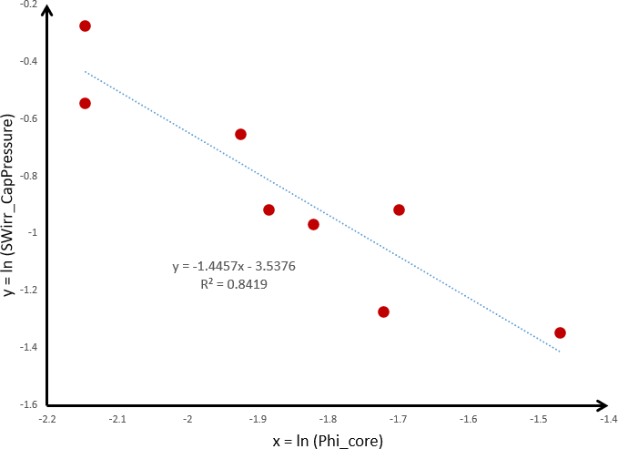
Linearized Holmes-Buckles log-log cross-plot of  (φ, SWirr)  core points from eight capillary pressure tests

The image below shows four functions available in GeolOil software to estimate a SWirr irreducible water saturation well log curve. The function (17) is the Holmes-Buckles correlation already discussed in this section. Notice that to the left of the min φ_lab box parameter, and to the right of max φ_lab box parameter, GeolOil will apply sigmoidal extensions that completely avoid overflow and underflow issues.

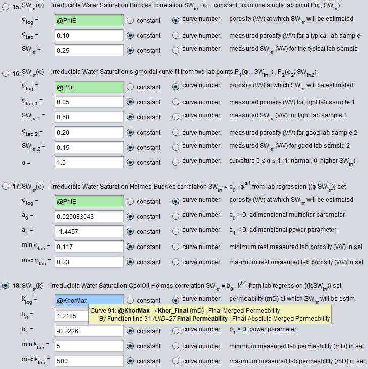
GeolOil software irreducible water saturation computations panel

How to estimate a well log curve of movable water saturation

Once that a SWirr (depth) curve has been estimated, the calculation of an approximate movable water saturation curve is immediate. Just estimate a SW(depth) water saturation curve from a standard SW model. Then, since the rock waters are either movable, or non movable (irreducible),  SW = SWirr + SW movable  ,  or:

SW movable  ≅   SW - SWirr

The log-plot of a gas reservoir below, shows estimated curves for SWirr irreducible water saturation, and SW_movable water saturation. Transition zones for gas-oil-water are also seen.

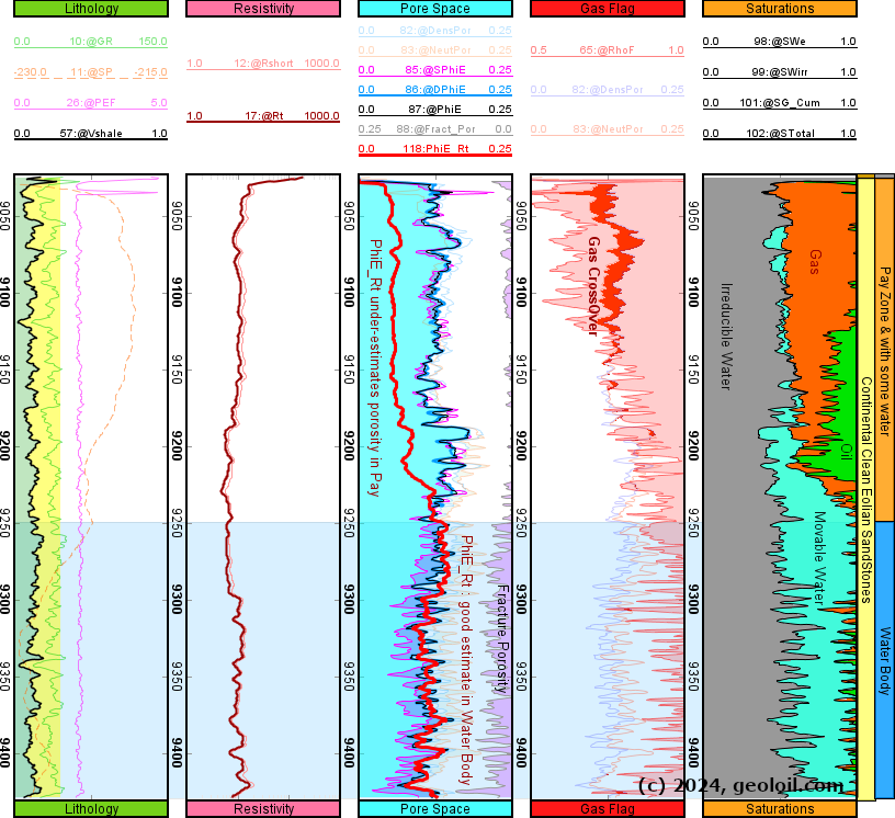
Log plot of a gas-oil reservoir showing curves for SWirr irreducible water saturation, and movable water saturation

Related articles: How to estimate porosity from Rxo flushed zone resistivity How to estimate water saturation from Rxo flushed zone resistivity How to estimate fracture porosity How to estimate the cementation porosity exponent m

© 2012-2023 GeolOil LLC. Please link or refer us under Creative Commons License CC-by-ND