


 TRAINING


 PAPERS
 REFERENCES
 GET IN TOUCH

|

|
 Downloads
|
 Prices
|
 Videos
|


How to define Rock Types from Bulk Volume of Water (BVW) and Wettability
By: Oscar Gonzalez, GeolOil LLC. This paper was first published on May 2025 on the website geoloil.com
A "rock type" scheme is a classification system of rocks at core plug or well-log scale size (inches), that groups rocks based on a similar fluid flow pattern behavior. It is also occasionally referred to by terms like litho-type or litho-facies.
⚠ Warning: The single-word term "facies" is sometimes used as a synonym for rock type. However, this nomenclature is ambiguous, as facies also refers to a large size scale (dozen or hundred of yards) classification of sedimentary environments.
Absolute permeability is often used as the main discriminatory variable to define rock types. However, it is not designed to take into account the interaction of the rock matrix with different fluids in multi-phase flows —just use relative permeability for that— Furthermore, absolute permeability values are seldom reliable or even available. In most cases, permeability is estimated from empirical data driven core-log correlations— usually noisy, poor ones, with low r2 determination coefficients.
This article presents a rock-type classification technique based on an attainable, conventional petrophysics well log interpretation outside of aquifers and water pockets. It is simply a 3D cross-plot that proved to be useful for a particular clastic reservoir studied. The three variables x, y, and z used in this template are the following:
- X: Effective Porosity. This variable explicitly captures the pore space storage capacity that may flow through the rock. It excludes trapped, unconnected pores inside clays. Effective porosity is a standard petrophysical computation from well logs. Besides fluid storage, porosity usually (not always) has some degree of correlation with permeability and fluid flow patterns. So, it may carry some "information" (weak or strong) or relationship with fluid flow, being a natural candidate variable for rock type schemes.
- Y: Volume of shale (Vshale or VSH). The nature, the arrangement, the fabric, the particle size, the amount, and the minerals present in the clays and silt usually affect the rock-fluid interaction. It also may drive the rock wettability or its affinity to be water-wet or oil-wet, thus affecting the fluid flow pattern and multi-phase flow. The joint (x,y) variables of effective porosity (PhiE), and Volume of shale (VSH), defines a 2D point expected to have some relationship with the flow behaviour.
- Z: A "response" or "dependent" variable z≅f(x,y) that succeeds to split the point collection into easily identifiable 2D partition group polygons. This Z variable is plotted using a color palette for easy visual identification. Variables for Z may describe for instance, how fluid phases may stick to water, oil or gas. Natural candidates for Z are water saturation, and bulk volume of water (BVW=PhiE*SW). In this study, BVW was found as the best discriminatory variable. The reason is not difficult to grasp. While water saturation describes the normalized (to porosity) proportion of water in the pore space, the BVW Bulk Volume of Water precisely measures how much water is stuck in the pores. A physically "tangible" property.
The images below show two 3D color palette cross-plots of x=effective porosity, y=Vshale, and z=water saturation or z=bulk volume of water. The 7,639 data points were collected from 65 wells of a clastic Wyoming reservoir.
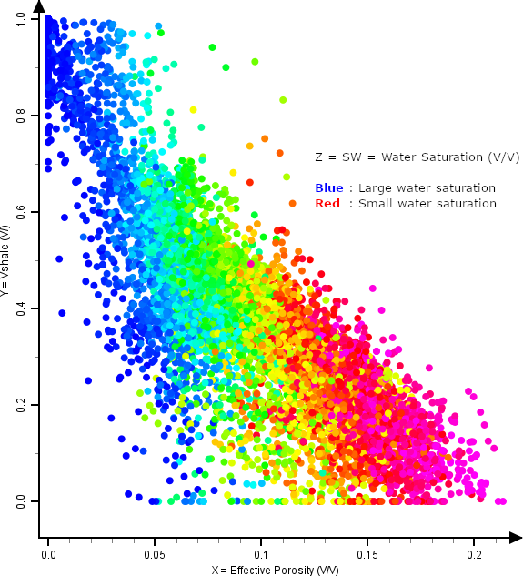
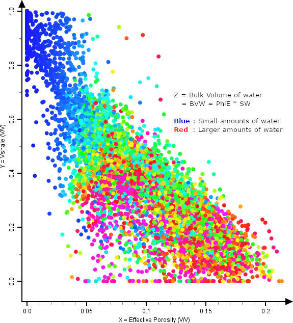
3D color palette cross-plots of x=Effective Porosity, y=Vshale, and Z=Water Saturation or Bulk Volume of Water
The first cross-plot based on z=SW water saturation, suggests that a classification based only on one variable x=effective porosity drives most of the SW heterogeneity or dispersion. That is, for a fixed porosity, the volume of shale variation slightly changes the water saturation.
The second cross-plot based on z=BVW Bulk Volume of Water, pops out more information. For instance, around a constant porosity of 8%, there is a big influence on how the shaliness changes the amount of water when VSH is above or below 45%. Since the porosity used is the effective porosity, the pore volume is the same when moving vertically through the y=VSH axis.
This behavior suggests that it is the electro-chemical nature of the clays that changes the amount of water —bulk volume of water— that sticks to the rock matrix. That is, it seems that the clays affect the rock wettability, allowing us to define four clear rock types:
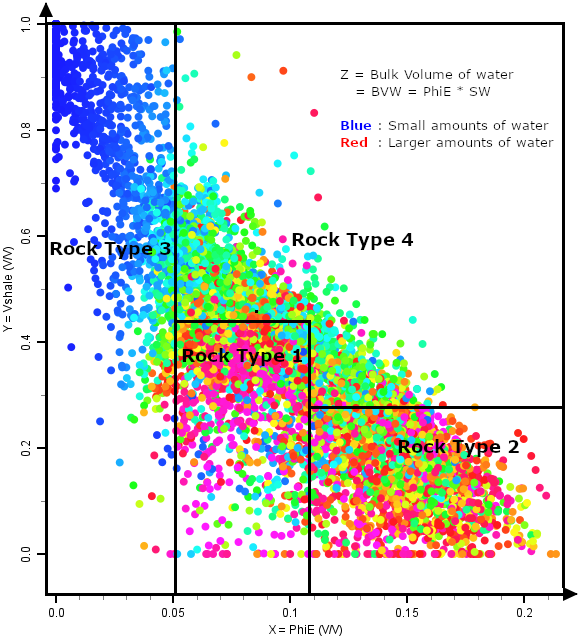
Rock-type classification cross-plot from porosity, Vshale, and BVW Bulk Volume of Water
 Notice that a qualitative high hue contrast, full range blue-red color scale for Z=BVW is enough to define the rock type polygons.
Once that each rock type has defined its own unique polygonal or 2D areal shape,
any 2D target rock point P(PhiE,Vshale) is classified onto a rock type
RTi if P ∈ Polygoni .
The Z=BVW values do no enter explicitly into the classification rule;
for instance, a point P(PhiE,Vshale) is classified as RT2 if (PhiE≥0.108) and
(Vshale≤0.27), the BVW value did not enter into the solved classification rule.
Notice that a qualitative high hue contrast, full range blue-red color scale for Z=BVW is enough to define the rock type polygons.
Once that each rock type has defined its own unique polygonal or 2D areal shape,
any 2D target rock point P(PhiE,Vshale) is classified onto a rock type
RTi if P ∈ Polygoni .
The Z=BVW values do no enter explicitly into the classification rule;
for instance, a point P(PhiE,Vshale) is classified as RT2 if (PhiE≥0.108) and
(Vshale≤0.27), the BVW value did not enter into the solved classification rule.
Since BVW=PhiE*SWe , the rock-type polygons are implicitly built as functions of three well log
variables, Polygoni = f(PhiE,Vhale,SWe), which encapsulates a lot of geological and petrophysical
information. Notice also that these three variables don't need
to be statistically nor petro-physically independent: In the cross-plot shown, PhiE and Vshale have a negative
Pearson's ρ
correlation dispersion coefficient. And also, SWe is related to PhiE through approximating equations like
Archie,
Simandoux,
Indonesia,
or other models.∎
The defined rock types can then be used to build a custom reservoir simulation model:
- Construct a 3D geo-cellular static model, using proper upscaling methods to handle different size scales from the well-log to the coarser static model.
- For each 3D cell in the static model, read their volumetrically upscaled values of effective porosity PhiE and Vshale. This defines a single 2D (PhiE, Vshale) point.
- Find where the 2D (PhiE, Vshale) point lies in the rock-type cross-plot. Pair each 3D cell with its corresponding rock type.
- Define a set of relative permeability curves per each rock type. Usually this is a manual trial and error process as relative permeability curves are seldom reliable or even available.
- Fine-tune fluid parameters and the relative permeability curves themselves until an acceptable fluid production rate history is matched for each well.
- Use the fitted simulation model to forecast future production for different exploitation schemes.

|
Related articles:
|
|
| |


|
|
|
© 2012-2026 GeolOil LLC. Please link or refer us under Creative Commons License CC-by-ND |