


 TRAINING


 PAPERS
 REFERENCES
 GET IN TOUCH

|

|
 Downloads
|
 Prices
|
 Videos
|


|
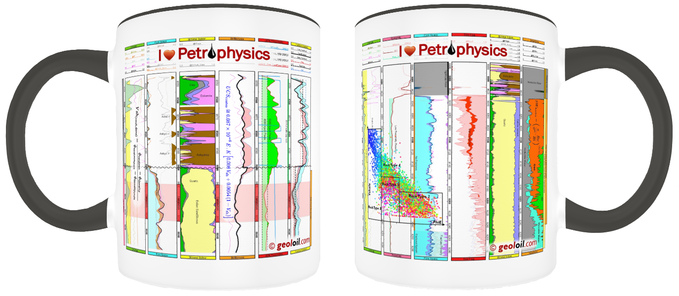
"I love Petrophysics" |
GeolOil - How to compute probabilistic well log curve uncertainty confidence bands
Any time a petrophysical property is measured in a laboratory, an inherent intrinsic uncertainty error is present. At each depth xi i=1,2,...,n , a property yi (like porosity) is measured from an extracted core plug. Hence the collection of {(xi, yi)}, i=1,2,...,n lab points can be plotted as a log curve for the well. If y=f(x) denotes the log curve as a function of depth x, a probabilistic model can be written as:
yi = f (xi) + εi i=1,2,...,n where εi is a random error.
The problem is to find quantile Q envelope confidence band functions gq(•) that embraces the function f(•) within a known probability. For example:
Prob { g25%(x) < f(x) < g75%(x) } = 75% - 25% = 50% defines a 50% confidence band, like the log plot shown below:
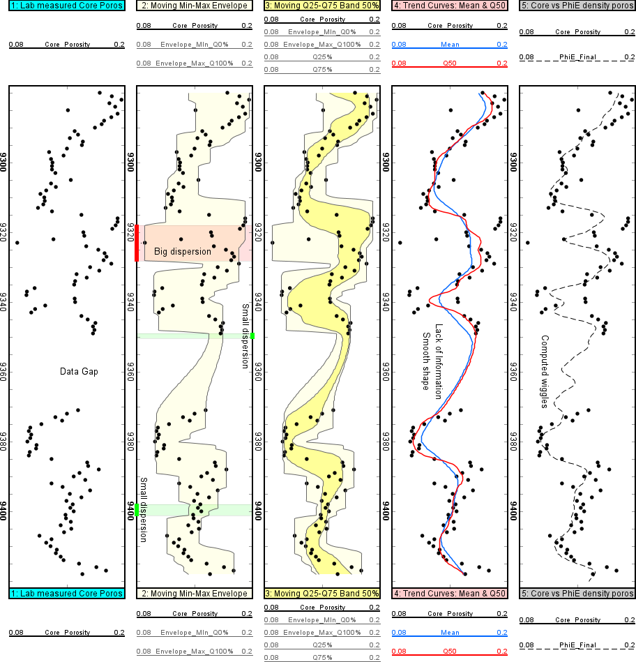
Probabilistic uncertainty curve confidence-bands for porosity core laboratory data, using a bandwidth of h=5 ft.
The method to compute confidence band functions should follow these three principles:
- The curves f(•) and g(•) must be non-parametric. That is, no functional form (like linear or polynomial) is assumed. The method should be self-content data-driven.
- The errors ε(x) must be also non parametric. That is, while ε can follow probability density functions with an expected value of E(ε(x))=0, no assumptions are made regarding the density shape. Likewise, no assumptions are made regarding the error variance Var(ε(x)). Hence the variance can be irregular or heteroscedastic. As an illustration, in the log plot shown below, the variance at the depth of 9,400 ft. (a narrow bottle-neck) is smaller than the heterogeneity variance around the depth of 9,325 ft.
- For each depth xi, normally only one measurement is available —so there is no strict possibility to perform a lack of fit test— This is quite common for petrophysical lab methods. Even if the measurement process is non-destructive, the lab protocol itself changes the physical core sample. Its wettability is changed when the sample is cleaned with toluene solvent, the pore space may have suffered induced cracks during pressure lab tests, etc.
The former three principles are quite general, and discard popular statistical techniques like well known ordinary least squares regression, and even non-parametric kernel regression. If it can be assumed that the variance Var(ε(x)) at a depth x is similar to the variance at the depths in a small neighborhood x ± h , then the set of the yi measurements that lie between xi ∈ ( x - h(x) , x + h(x)) is a local sample of the probability distribution of f(•) around the depth x.
In the log plot shown above, the blue first track shows core porosity measurement values with a large data gap around the depths of 9,360 ft. The pale yellow second track shows a moving 100% confidence band that completely wraps all the core points between a minimum Q0% quantile envelope (the "minimum") curve, and a Q100% quantile envelope curve (the "maximum"). Notice that the band is somewhat jagged, and albeit similar, it is not a convex hull, but an approximate probability confidence band.
The yellow third track shows a moving 50% confidence band, completely embedded inside the wider 100% confidence band. Around 50% of the points lie inside the band. The pink fourth track compares the core data against central trends defined by a Q50% quantile curve, and a moving average curve. Around the 9,360 ft zone of data gap, none of the methods succeed to capture an informative detailed shape, but a general smoothed trend. The gray last track compares the core lab data against a deterministic curve computed by the density porosity equation. Notice how the curve now brings an informative wiggle shape around the depths of 9,360 ft, as it uses log data of the bulk density curve available at those depths.
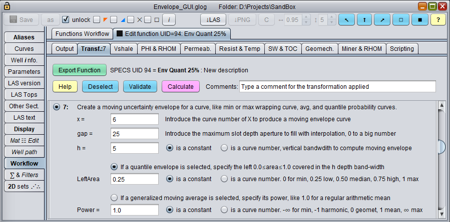
GUI Panel to compute an uncertainty Q25% confidence curve for porosity core laboratory data

|
Related article:
|
|
| |


|
|
|
© 2012-2026 GeolOil LLC. Please link or refer us under Creative Commons License CC-by-ND |