Absolute permeability is one of the most difficult petrophysical properties to model from well log data. The essential problem is that permeability is related to pore throat size rather than the volumetric proportion of connected void space in the rock (effective porosity). So rocks with a same porosity can perfectly have different values of permeability. To add more complexity to the problem, permeability is usually a very heterogeneous property that easily spans over three or even five orders of magnitude in many typical reservoirs.

While porosity can be estimated from regular well log curves, like bulk density and neutron porosity, a log permeability estimate (at curve resolution size) would require curves from NMR Nuclear Magnetic Resonance tools. Since there is a general weak trend that high porosities also show larger pore sizes, correlations are built for permeability as empirical functions of porosity for each rock type  k ≅ f(φ). Then, the function f(φ) is applied to the continuous porosity log curve, and a continuous permeability curve is produced for the well.

Core lab measurements that collect paired values of porosity and maximum horizontal permeability (x=φ, y=KhMax) are cross-plotted and the empirical correlation f(φ) is adjusted to the dispersed points. Even after carefully splitting the core samples into several rock types and remove unreliable and influential outliers, adjusted r²  determination coefficients are typically low, around 15% to only 65%.

There are many reasons for these weak correlations:

When fitting empirical f(φ) correlations as univariate functions of the porosity φ, the following functional form, has historically yielded reasonable results:

k = b₀ . φ^b1

The form is converted into a linear expression   y=c₀+c₁x   on   x and y   by taking natural logarithms:

ln(k) = c₀ + c₁.ln(φ)     where:   y=ln(k)    c₀=ln(b₀)    c₁ =b₁   and    x=ln(φ)

A set of  i=1,2,..,n core lab sample measurements of porosity and permeability  {(φ_i, k_i)}  is then converted to a set of  {(x_i, y_i)}  points and then the parameters c₀ and c₁  can be estimated with techniques like ordinary least squares regression. However, since both x and y are random variables suffering lab errors, —least squares assumption works when y is a random variable, but x is not— a more correct solution is found using Deming orthogonal regression. Its probabilistic solution is:

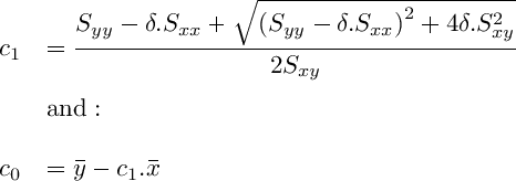
Where:

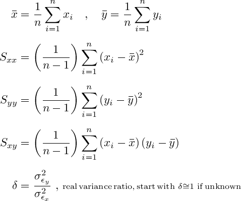
Beyond the one to one univariate porosity-permeability simple correlation discussed, there is no reason why other regressor variables can't be added to enrich and increase the adjusted determination coefficient r². The figure below shows the GeolOil work-flow panel with some built-in permeability correlations from core data.

The GeolOil software panel with major built-in permeability correlations from core data

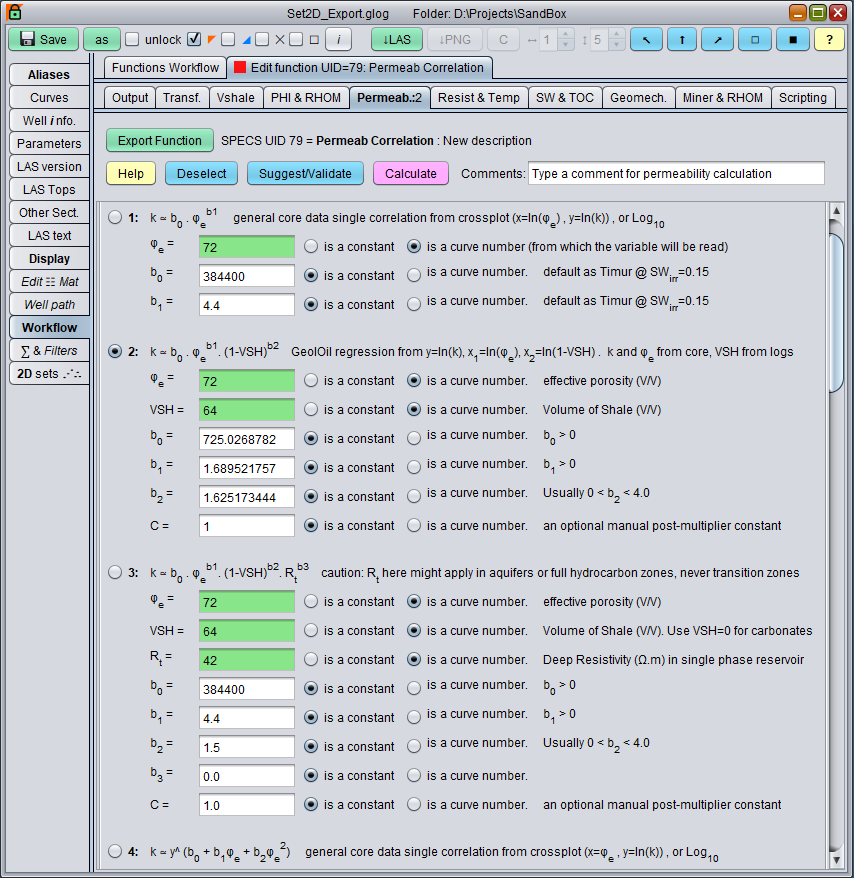
A particularly interesting equation is the second one in the above panel. It establishes a multiple regression of permeability as a join function with both porosity and volume of shale VSH:   k = b₀ . φ^b1 . (1-VSH)^b2

The linearized equation (in the coefficients a₀, a₁, and a₂), can be applied on clastic reservoirs from easily accessible conventional data: permeability and porosity from core laboratory measurements, but VSH shaliness estimated from well log curves (like a Vshale estimated from gamma ray, or from neutron to density porosity difference). In most of the cases, the inclusion of the VSH term, slightly but steadily increases the adjusted determination coefficient, improving the permeability range response compared with a flatter behaviour of a porosity only term equation. The effects of the porosity and shaliness terms on permeability can be interpreted as follows:

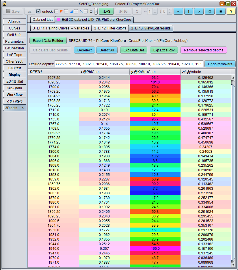
The GeolOil core data selection panel to export results to an Excel spreadsheet

The above panel shows the expected general relationships discussed for core data from a clastic reservoir. The maximum horizontal permeability KhMaxCore is highlighted with saturated colors at the center column. Comparing the with the left PhiCore column, it can be seen matching color behaviours: warm red tones like reds in permeability are paired with warm red tones in porosity, and blue tones with blues and greens. Likewise, an inverse color relationship is observed with the right column Vshale, permeability warm colors like reds are paired with blues and green colors, and vice versa.

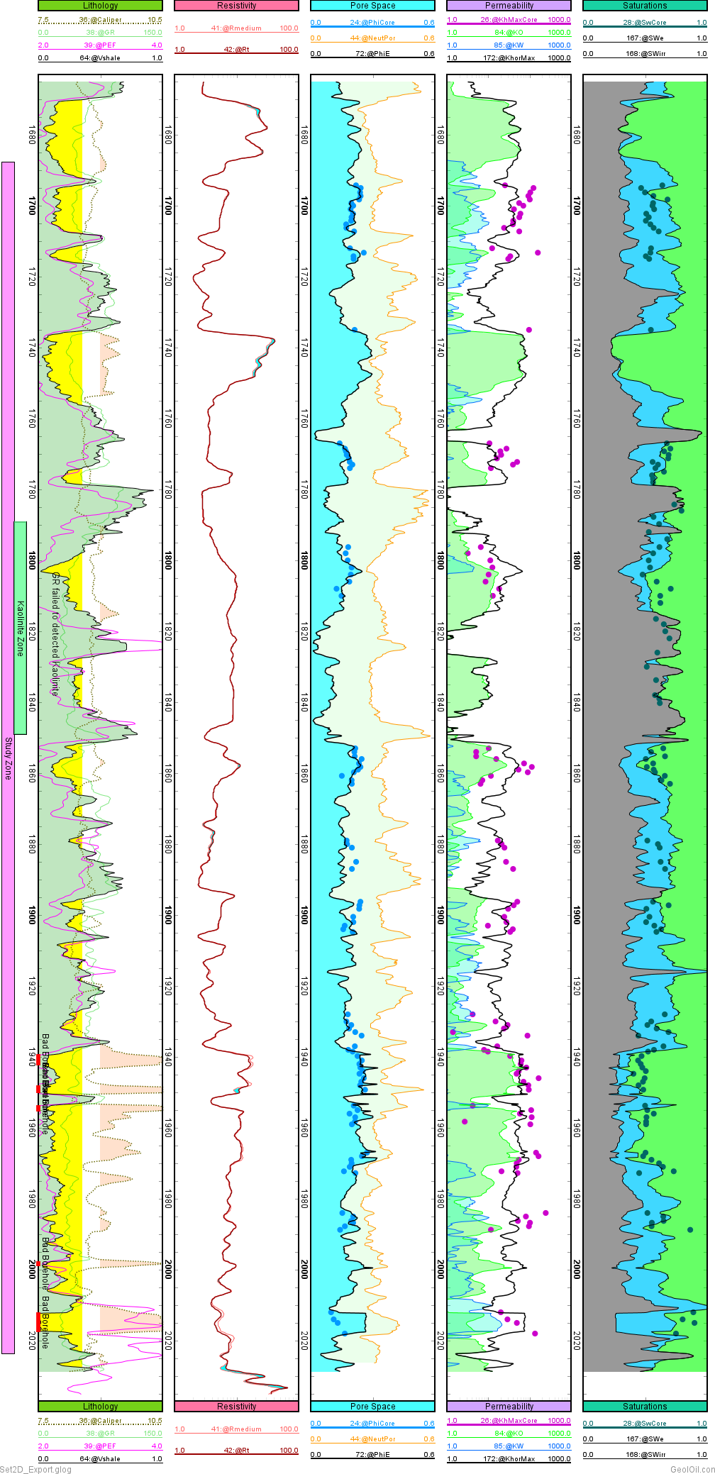
Well log plot from a clastic reservoir with permeability and porosity core data

The corresponding well log plot is shown in the image above. Although the curves and core data quality are not the best, it displays other interesting features. The permeability track shows the core data points together with the continuous black curve of absolute permeability computed from the fitted equation   k = b₀ . φ^b1 . (1-VSH)^b2   and also the permeabilities KO and KW to Oil (green) and Water (blue) respectively. Notice a good match behaviour of KW with the free movable water estimate (the difference between SWe and SWirr curves) at the right most saturations track (the blue filling).

The next figure shows the fitted permeability equation computed with Excel after exporting the CSV data. Although the overall r² fit value is low, it shows the expected behaviour. Notice also that all the green regression P-values are highly significant (less than 1%), so the terms Phi and VSH legit-amiable enter into the model with valid statistical contributions.

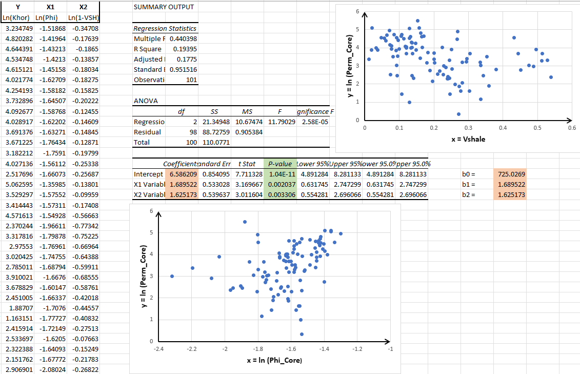
Fitted model of permeability versus porosity and Vshale

	Related article: How to learn petrophysics by practicing with log log interpretation examples.
	Related video: How to export well log curves to Excel

GeolOil is listed by the official SPWLA software directory

© 2012-2024 GeolOil LLC. Please link or refer us under Creative Commons License CC-by-ND